\[ \newcommand{\bs}{\boldsymbol} \newcommand{\bsX}{\boldsymbol{X}} \newcommand{\bf}{\mathbf} \newcommand{\msc}{\mathscr} \newcommand{\mca}{\mathcal} \newcommand{\T}{\text{T}} \newcommand{\rme}{\mathrm{e}} \newcommand{\rmi}{\mathrm{i}} \newcommand{\rmj}{\mathrm{j}} \newcommand{\rmd}{\mathrm{d}} \newcommand{\rmm}{\mathrm{m}} \newcommand{\rmb}{\mathrm{b}} \newcommand{\and}{\land} \newcommand{\or}{\lor} \newcommand{\exist}{\exists} \newcommand{\sube}{\subseteq} \newcommand{\lr}[3]{\left#1 #2 \right#3} \newcommand{\intfy}{\int_{-\infty}^{+\infty}} \newcommand{\sumfy}[1]{\sum_{#1=-\infty}^{+\infty}} \newcommand{\vt}{\vartheta} \newcommand{\ve}{\varepsilon} \newcommand{\vp}{\varphi} \newcommand{\Var}{\text{Var}} \newcommand{\Cov}{\text{Cov}} \newcommand{\edef}{\xlongequal{def}} \newcommand{\prob}{\text{P}} \newcommand{\Exp}{\text{E}} \newcommand{\t}[1]{\text#1} \newcommand{\N}{\mathbb{N}} \newcommand{\Z}{\mathbb{Z}} \newcommand{\Q}{\mathbb{Q}} \newcommand{\R}{\mathbb{R}} \newcommand{\C}{\mathbb{C}} \newcommand{\versionofnewcommand}{\text{260125}} \]

Adaptation and Firing Patterns

The stereotypical arrangement of inter-spike intervals defines the neuronal firing pattern. Diversity of firing patterns can be explained by adaptation mechanisms, which is in turn depend on the zoo of ion channels and neuronal anatomy.

However, a single equation characterized by a function $f(u)$, can not sufficiently describe adaptation mechanism. The membrane voltage has to be coupled with an/some abstract adaptation current $w$, or $w_k$ for multiple adaptation current. Let's take adaptive exponential integrate-and-fire model as an example.

Adaptive Exponential Integrate-and-Fire

Based on exponential IF model, the adaptive exponential integrate-and-fire model (AdEx) is given as:

\[ \begin{aligned} &\tau_m\frac{\rmd u}{\rmd t}=-(u-u_\rest)+\Delta_T\exp\lr({\frac{u-\vthrh}{\Delta_T}})-Rw+RI(t)\\ &\tau_w\frac{\rmd w}{\rmd t}=a(u-u_\rest)-w+b\tau_w\sum_{t^f}\delta(t-t^f) \end{aligned} \]

In which parameter $a$ describes the coupling of $u$ and $w$, while $b$ describes the contribution of each spike to dynamics of $w$. And the $-w$ term indicates that, $w$ has a motivation to go back to zero.

The AdEx model is capable of reproducing a large variety of firing patterns. We will discuss this issue in subsequent sections.

Firing Patterns

Classification of Firing Patterns

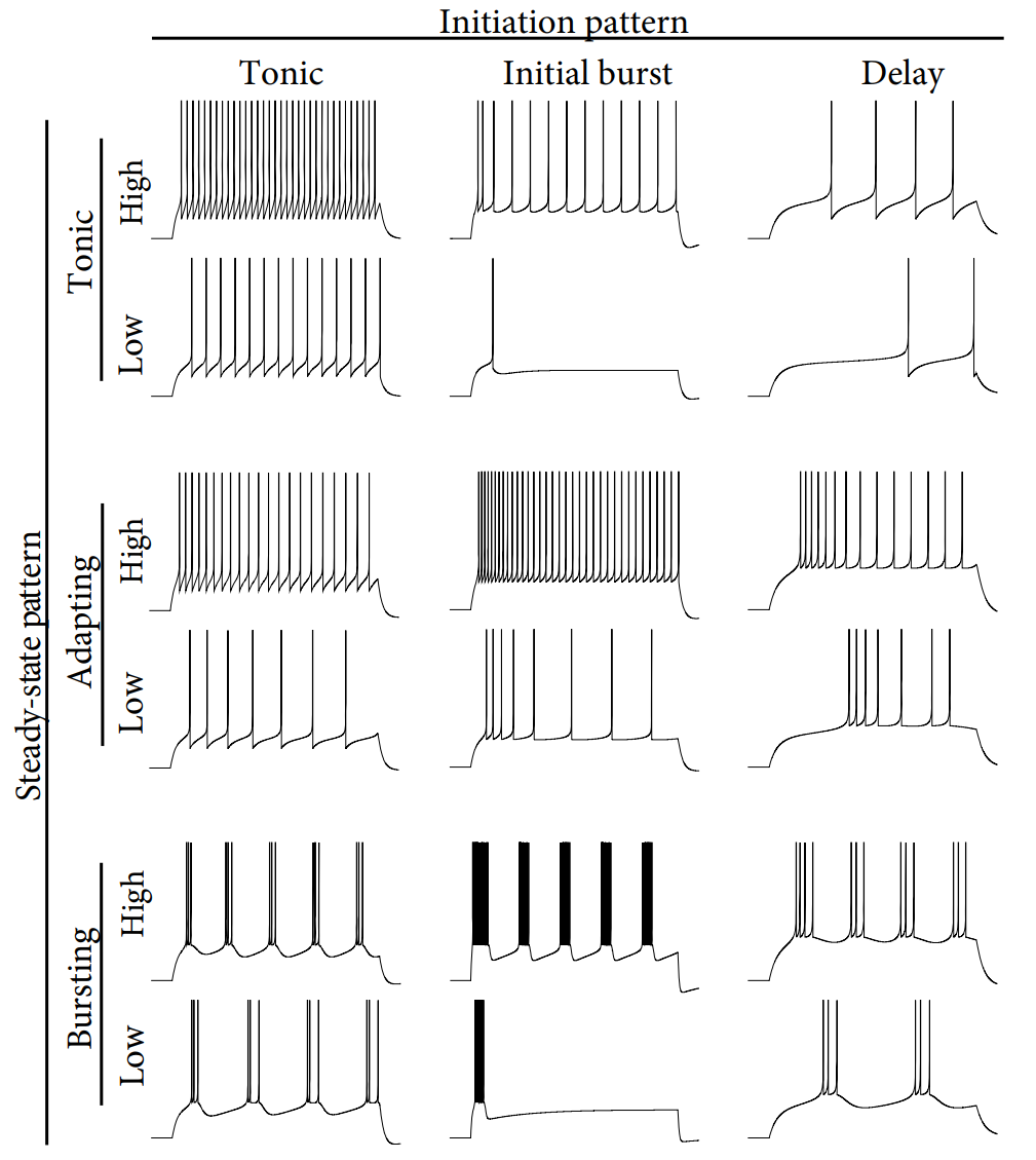
If we consider the firing pattern right after the onset of current input, which refers to initial transient phase, three main initial patterns can be found:

tonic: the initiation cannot be distinguished from the rest of the spiking response
initial burst: frequency of initial respond is significantly greater than that of the steady state
delay: the firing initiates with a delay

After the initiation transient, the neuron exhibits a steady-state pattern. There are also three main types:

tonic: evenly spaced spikes
adapting: gradually increasing inter-spike intervals.
bursting: regular alternations between short and long inter-spike intervals.

Figures of all these firing patters are provided below:

All of those patters can be generated through adjusting parameters in the equations, as below:

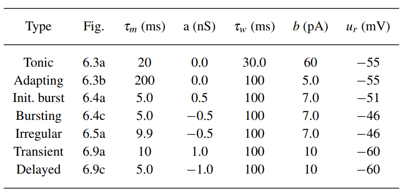
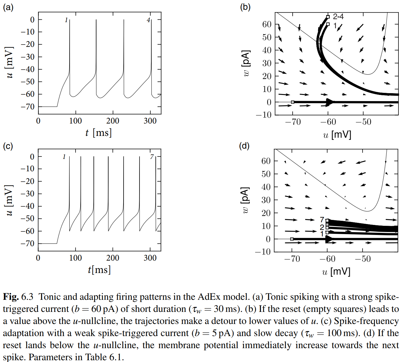
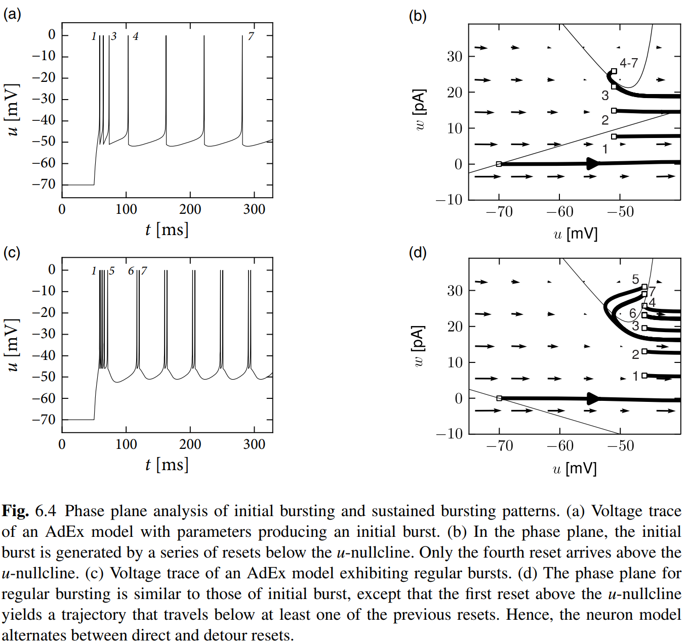
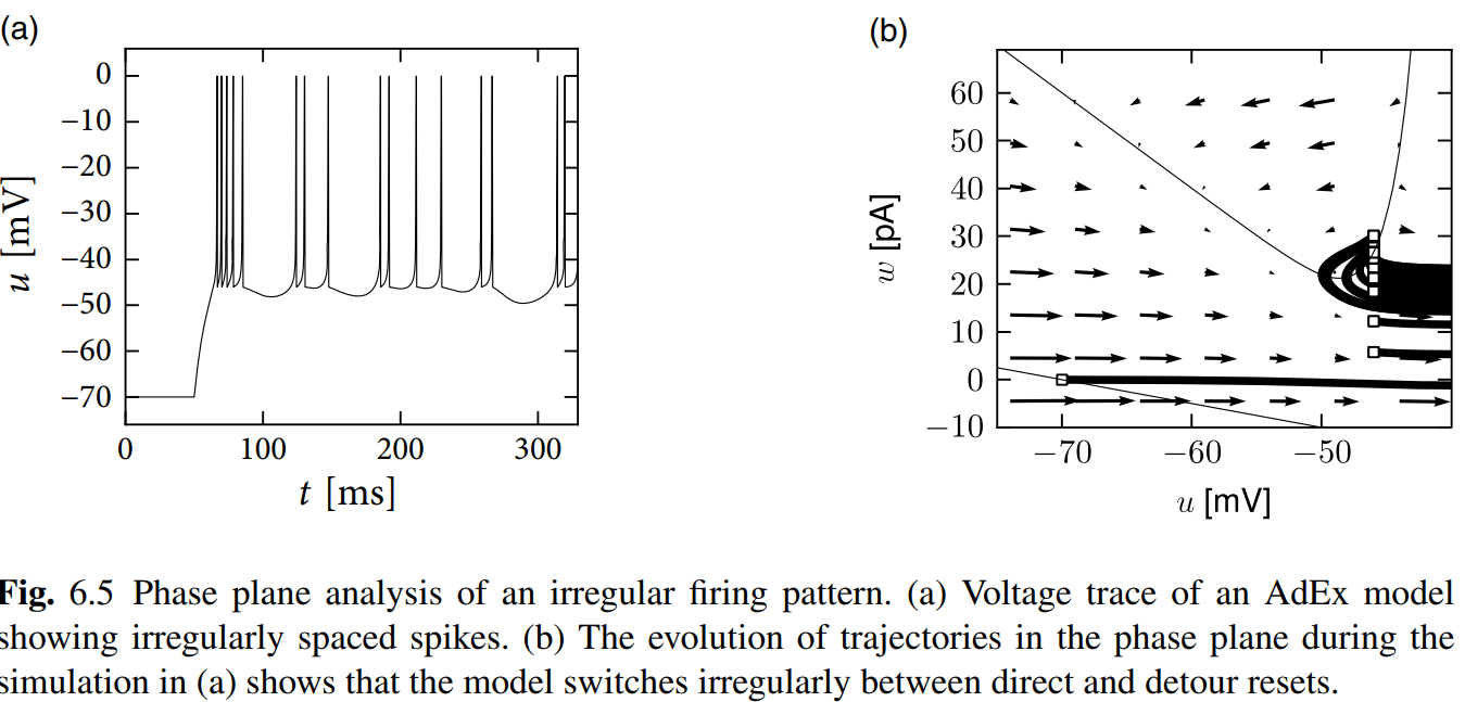
Phase Plane Analysis of Nonlinear Integrate-and-Fire Models in Two Dimensions

Just read these figures and enjoy the progress that finding how the tonic, adapting, initial bursting and bursting generate with different parameters. Hand-drawing is highly recommended!

Biophysical Origin of Adaptation

Subthreshold adaptation by ion channel: the variable $w$

Now, biophysical interpretation of parameter $a,\tau_w$ has not been unveiled. We have known that the dynamics around $u_\rest$ approximately takes a linear form, which is useful for simplify our analysis of properties of parameters. In order to treat it more generally, we replace $u_\rest$ with $E_0$:

\[ \tau_w\frac{\rmd w}{\rmd t}=a(u-E_0)-w \]

Remember that in Chapter 4, in 2D HH model, we introduced a parameter by the same notation $w$, where $w$ represents the combination of $h$ and $n$. The feasibility of this simulation derives from the similarity of their time course behavior, and the dynamical time scale separation of $h,\ n$ and $m$. Actually, $w$ in adaptation models also represents the other channels which have a slower dynamics, on contrary to sodium channel. Thus, let us take potassium channel in HH model for an example:

\[ \begin{aligned} \tau_m&\frac{\rmd u}{\rmd t}=-(u-E_L)-R_L\ g_K\ n^p (u-E_K)+R_LI_{\t{ext}}\\ &\frac{\rmd n}{\rmd t}=-\frac{n-n_0(u)}{\tau_n(u)} \end{aligned} \]

Consider a linearized form by approximating the parameters around the rest potential $E_0$, which is a fixed point: ($I_\t{ext}$ is set to zero.)

\[ \begin{cases} \dot{u}=0\\ \dot{n}=0 \end{cases} \ \Rightarrow\ \begin{cases} (E_0-E_L)-R_L\ g_K\ n^p(E_0-E_K)=0\\ n=n_0(E_0) \end{cases}\\ \]

which gives:

\[ E_0=\frac{E_L+(R_L\ g_K)[n_0(E_0)]^pE_K}{1+(R_L\ g_K[n_)(E_0)^p])} \]

We introduce a parameter $\beta$, taking a form as below:

\[ \beta= g_K\lr({p\ [n_0(E_0)]^{p-1}})(E_0-E_K) \]

and linearly expand $n_0(u)$:

\[ n_0(u)=n_0(E_0)+\frac{\rmd}{\rmd t}n_0(u-E_0) \]

Thus, our adorable spirit, the magical parameter $w$ emerges:

\[ w=\beta\ [n(u)-n_0(E_0)] \]

which gives the equation:

\[ \tau_n(E_0)\frac{\rmd w}{\rmd t}=a(u-E_0)-w \]

The parameter $a$ is proportional to the sensitivity of the channel to a change in the membrane voltage, as measured by the slope $\rmd n_0/\rmd u$ at the equilibrium potential $E_0$.

Subthreshold Adaptation by Passive Dendrites

Let us simplify a neuron by considering it with two compartments, the soma, and the dendrite, corresponding to subscripts $\text{s}$ and $\t{d}$ respectively. Then, the equation of this model is:

\[ \begin{aligned} &\frac{\rmd V^\t{s}}{\rmd t}=\frac{1}{C^\t{s}}\lr[{-\frac{(V^\t{s}-u_\rest)}{R_\t{T}^\t{s}}-\frac{V^\t{s}-V^\t{d}}{R_\t{L}}+I(t)}]\\ &\frac{\rmd V^\t{d}}{\rmd t}=\frac{1}{C^\t{d}}\lr[{-\frac{(V^\t{d}-E^\t{d})}{R_\t{T}^\t{d}}-\frac{V^\t{d}-V^\t{s}}{R_\t{L}}}] \end{aligned} \]

Let $w$ represents the current flowing from the dendrite into the soma, and assume that $E^\t{d}=u_\rest=E$,

\[ w=-\frac{V^\t{d}-u_\rest}{R_\t{L}}=-\frac{V^\t{d}-E}{R_\t{L}} \]

Dynamics of potential change in soma can be written as a form similar to equations discussed above:

$$ \begin{aligned} &\frac{\rmd V^\t{s}}{\rmd t}=\frac{1}{C^\t{s}}\lr[{-\frac{(V^\t{s}-u_\rest)}{R_\t{T}^\t{s}}-\frac{V^\t{s}-V^\t{d}}{R_\t{L}}}]\ \Leftrightarrow\ C^\t{s}&\frac{\rmd V^\t{s}}{\rmd t}={-\frac{(V^\t{s}-E)}{R_\t{T}^\t{s}}-\frac{V^\t{s}-V^\t{d}}{R_\t{L}}}\ \Leftrightarrow C^\t{s}&\frac{\rmd V^\t{s}}{\rmd t}= -\lr({\frac{V^\t{s}}{R_\t{T}^\t{s}}+\frac{V^\t{s}}{R_\t{L}}}) +\lr({\frac{E}{R_\t{T}^\t{s}}+\frac{E}{R_\t{L}}}) +\lr({\frac{V^\t{d}}{R_\t{L}}-\frac{E}{R_\t{L}}})\ \Leftrightarrow C^\t{s}\frac{R_\t{T}^\t{s}R_\t{L}}{R_\t{T}^\t{s}+R_\t{L}} \cdot&\frac{\rmd V^\t{s}}{\rmd t}= -\lr({V^\t{s}-E})-\frac{R_\t{T}^\t{s}R_\t{L}}{R_\t{T}^\t{s}+R_\t{L}}\cdot w

\end{aligned} $$

Set $R^{\t{eff}}={R_\t{T}^\t{s}R_\t{L}}/\lr({R_\t{T}^\t{s}+R_\t{L}})$, and $\tau^{\t{eff}}=R^{\t{eff}}C$, then:

\[ \tau^{\t{eff}}\frac{\rmd V^{\t{s}}}{\rmd t}=-(V^\t{s}-E)-R^{\t{eff}}w \]

As for dynamics of $w$,

\[ \begin{aligned} \frac{\rmd w}{\rmd t}&=-\frac{1}{R_\t{L}}\frac{\rmd V^\t{d}}{\rmd t}\\ \Leftrightarrow \frac{\rmd w}{\rmd t}&=-\frac{1}{R_{\t{L}}C^\t{d}} \lr[{-\frac{(V^\t{d}-E^\t{d})}{R_\t{T}^\t{d}} -\frac{V^\t{d}-V^\t{s}}{R_\t{L}}}]\\ \Leftrightarrow {R_{\t{L}}C^\t{d}}\frac{\rmd w}{\rmd t}& =-{\frac{V^\t{s}-E}{R_\t{L}}+\frac{V^\t{d}-E}{R_\t{L}}} +\frac{V^\t{d}-E}{R_\t{T}^\t{d}}\\ \Leftrightarrow {R_{\t{L}}C^\t{d}}\frac{\rmd w}{\rmd t}& =-{\frac{V^\t{s}-E}{R_\t{L}}}-\lr({1+\frac{R_\t{L}}{R_\t{T}^\t{d}}})w\\ \Leftrightarrow \frac{R_\t{T}^\t{d}R_\t{L}}{R_\t{T}^\t{d}+R_\t{L}}{C^\t{d}} \frac{\rmd w}{\rmd t}& =-\frac{R_\t{T}^\t{d}}{\lr({R_\t{T}^\t{d}+R_\t{L}})R_\t{L}} \lr({V^\t{s}-E})-w\\ \end{aligned} \]

Set $a=-R_\t{T}^\t{d}/\lr({R_\t{T}^\t{d}+R_\t{L}})R_\t{L}$, and $\tau_{w}=R_\t{T}^\t{d}R_\t{L}{C^\t{d}}/\left({R_\t{T}^\t{d}+R_\t{L}}\right)$, then:

\[ \tau_w\frac{\rmd w}{\rmd t}=a(V^{\t{s}}-E)-w \]

There we get the full equations:

\[ \begin{aligned} \tau^{\t{eff}}\frac{\rmd V^{\t{s}}}{\rmd t}&=-(V^\t{s}-E)-R^{\t{eff}}w\\ \tau_w\frac{\rmd w}{\rmd t}&=a(V^{\t{s}}-E)-w \end{aligned} \]

Properties of Adaptation Caused by Passive Dendrites

Firstly, $a$ is always negative, which gives a motivation to facilitate subthreshold coupling.

Spike Response Model (SRM)

Remember that in Chapter 1, we had discussed a convolution form of membrane potential. That is,

\[ V(t)=u(t)-u_\rest=\int_0^{+\infty}\eta(s)S(t-s)\text{d}s+\int_0^{+\infty}\kappa(s)I(t-s)\text{d}s \]

Where $\eta(s)$ describes the reset current, while $\kappa(s)$ describes the time course of the voltage response to a short current impulse at time $s=0$.

Dynamic Threshold

SRM is based on the LIF model, but the threshold $\vartheta$ is not fixed, but time-dependent. Here is a standard model of the dynamic threshold:

\[ \vartheta(t)=\vartheta_0+\int_0^\infty \theta_1(s)S(t-s)\rmd s\ , \]

where $\vartheta_0$ is the "normal" threshold in the absence of spiking. Obviously, it takes the form same as $\int_0^{+\infty}\eta(s)S(t-s)\text{d}s$. Thus we can eliminate the time dependence of $\vartheta$ by:

\[ \begin{aligned} &\eta^{\t{eff}}(t)=\eta(t)-\vartheta(t)\\ \end{aligned} \]

or from the other hand, eliminating the time dependence of $\eta$:

\[ \vartheta(t)=\eta(t)-\eta^{\t{eff}}(t) \]

With this combination, it is easy to predict spike times $t^f$. Firstly, $h(t)=\int_0^{\infty}\kappa(s)I(t-s)\rmd s$ takes a simple form of convolution, where both the kernel function $\kappa$ and input $I$ are easy to calculate, different from the spike train $S(t)=\sum_f\delta(t-t^f)$. So, if we integrate the spike-afterpotential kernel $\eta$ into threshold $\vartheta$:

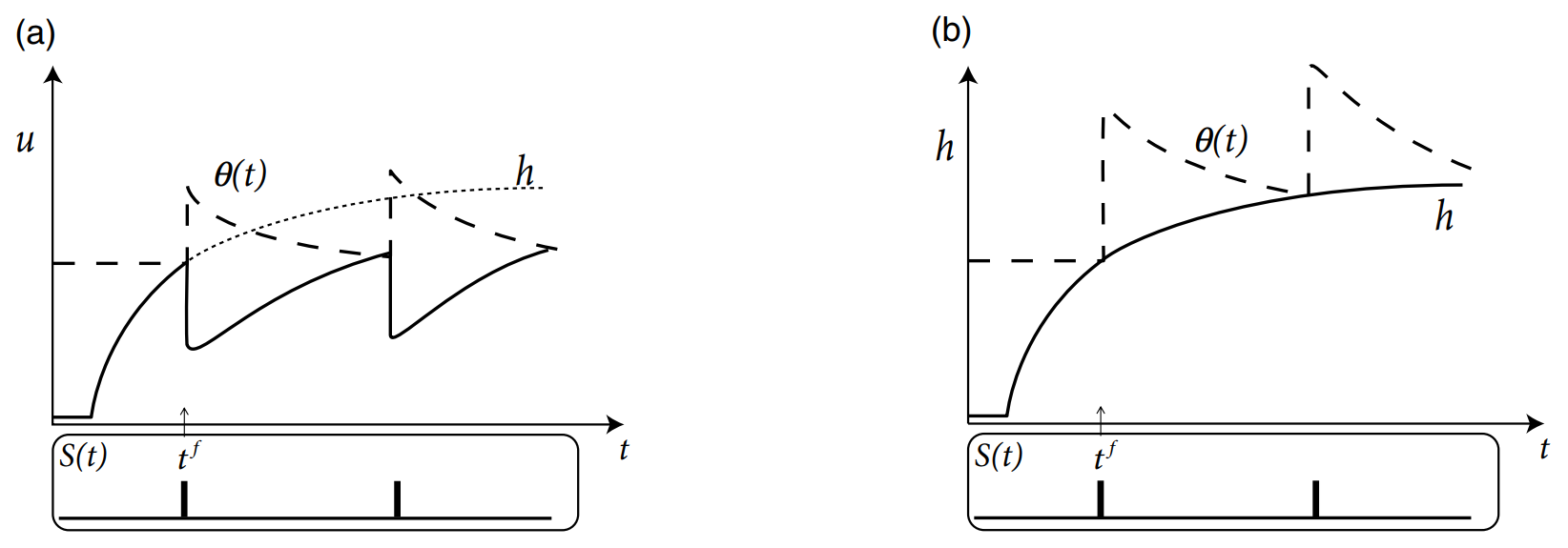
\[ \begin{aligned} &&u(t)=\int_0^{+\infty}\eta(s)S(t-s)\text{d}s+h(t)\quad&\t{reaches}\quad \vartheta(t)=\vartheta_0+\int_0^\infty \theta_1(s)S(t-s)\rmd s \\ &\to &u^{\t{eff}}(t)=h(t)\quad&\t{reaches}\quad \vartheta(t)=\vartheta_0+\int_0^{+\infty}[\theta_1(s)-\eta(s)]S(t-s)\text{d}s \end{aligned} \]

Just like figure (b) above, it is rather easier to predict $t^f$ than figure (a).

Mapping the Integrate-and-Fire Model to SRM

Adaptation variables $w_k$ can also be combined with LIF model:

\[ \begin{aligned} \tau_m\frac{\rmd u}{\rmd t}&=-(u-u_{\rest})-R\sum_kw_k+RI(t)\\ \tau_k\frac{\rmd w_k}{\rmd t}&=a(u-u_\rest)-w_k+b_k\tau_k\sum_{t^f}\delta(t-t^f) \end{aligned} \]

Let us define "output" current as:

\[ I^{\t{out}}(t)=-C(\vartheta-u_{\t{r}}) \sum_{f}\delta({t-t^f}) \]

which represents the reset current.

Multi-Compartment Integrate-and-Fire Model as an SRM

In this section, we want to show that neurons with a linear dendritic tree and a voltage threshold for spike firing at the soma (that is, neurons with spatial properties) can be mapped to the SRM.

To be continued...