\[ \newcommand{\bs}{\boldsymbol} \newcommand{\bsX}{\boldsymbol{X}} \newcommand{\bf}{\mathbf} \newcommand{\msc}{\mathscr} \newcommand{\mca}{\mathcal} \newcommand{\T}{\text{T}} \newcommand{\rme}{\mathrm{e}} \newcommand{\rmi}{\mathrm{i}} \newcommand{\rmj}{\mathrm{j}} \newcommand{\rmd}{\mathrm{d}} \newcommand{\rmm}{\mathrm{m}} \newcommand{\rmb}{\mathrm{b}} \newcommand{\and}{\land} \newcommand{\or}{\lor} \newcommand{\exist}{\exists} \newcommand{\sube}{\subseteq} \newcommand{\lr}[3]{\left#1 #2 \right#3} \newcommand{\intfy}{\int_{-\infty}^{+\infty}} \newcommand{\sumfy}[1]{\sum_{#1=-\infty}^{+\infty}} \newcommand{\vt}{\vartheta} \newcommand{\ve}{\varepsilon} \newcommand{\vp}{\varphi} \newcommand{\Var}{\text{Var}} \newcommand{\Cov}{\text{Cov}} \newcommand{\edef}{\xlongequal{def}} \newcommand{\prob}{\text{P}} \newcommand{\Exp}{\text{E}} \newcommand{\t}[1]{\text#1} \newcommand{\N}{\mathbb{N}} \newcommand{\Z}{\mathbb{Z}} \newcommand{\Q}{\mathbb{Q}} \newcommand{\R}{\mathbb{R}} \newcommand{\C}{\mathbb{C}} \newcommand{\versionofnewcommand}{\text{260125}} \]

Nonlinear Integrate-and-Fire Models

In a nonlinear integrate-and-fire model with a single variable \(u\), the membrane potential evolves according to:

\[ \tau\frac{\rmd u}{\rmd t}=f(u)+R(u)I \]

事实上, standard leaky integrate-and-fire model 正是它的退化形式:

\[ \tau\frac{\rmd u}{\rmd t}=u-u_{\rest}+RI \]

上式可以通过 scaling 变得更简单. 设:

\[ \begin{aligned} \tilde{u}(t) &=\tau\int_0^{u(t)}\frac{\rmd x}{R(x)}\\ \Rightarrow \frac{\rmd \tilde{u}}{\rmd t} &=\tau\cdot\frac{1}{R(u)}\frac{\rmd u}{\rmd t} \end{aligned} \]

这样就有:

\[ f(u)+R(u)I=\tau\frac{\rmd u}{\rmd t}=R(u)\cdot\frac{\rmd \tilde{u}}{\rmd t}\\ \]

如果定义 \(d(\tilde{u})=f(u)/R(u)\), 注意这里的 \(d\) 不是微分符号 \(\rmd\), 就有简单形式:

\[ \frac{\rmd{\tilde{u}}}{\rmd t}=d(\tilde{u})+I(t) \]

Exponential Integrate-and-Fire Model

Fourcaud-Trocme et al. gives the exponential integrate-and-fire model in 2003:

\[ \tau\frac{\rmd u}{\rmd t}=-(u-u_{\rest})+\Delta_T\exp\lr({\frac{u-\vartheta_{\t{rh}}}{\Delta_T}})+RI \]

\(\Delta_T\) 可以理解为 "sharpness" of the threshold. 对 \(f(u)\) 简单求可导可以发现, \(\Delta_T\) 越小, 在 \(\vartheta_{\text{rh}}\) 处拐弯的速度就越大, 也就是越 "sharp". 如下图所示:

\[ \frac{\rmd}{\rmd u} f(u)=\exp\lr({\frac{u-\vartheta_{\text{rh}}}{\Delta_T}})-1 \]

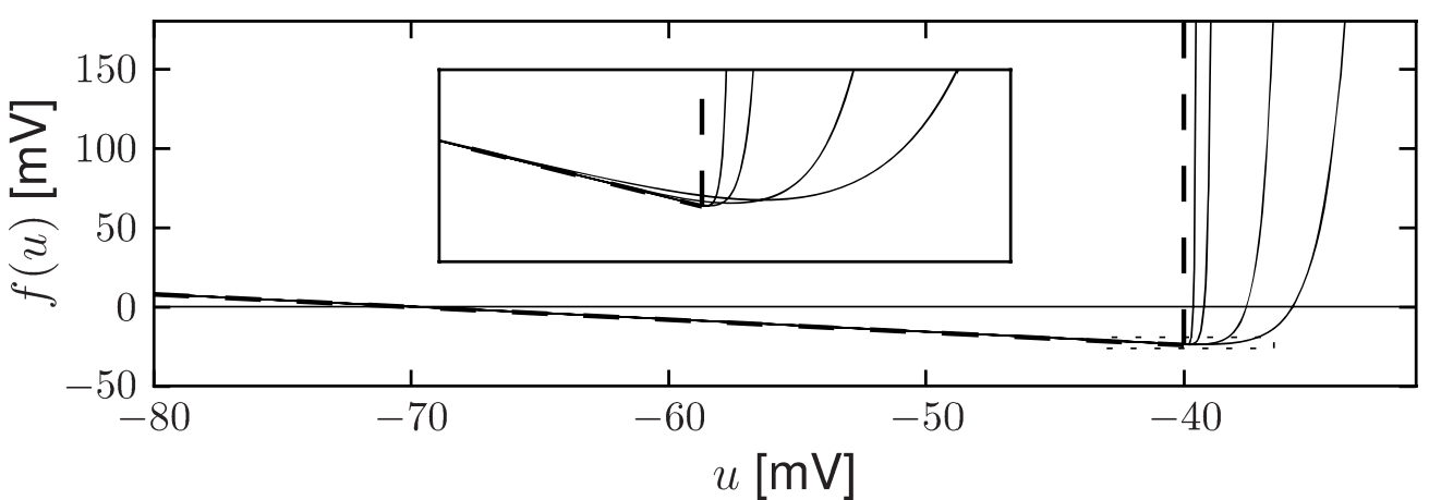
特别地, 如上图中虚线所示, 当 \(\Delta_T\to0\) 时, 指数项退化为 \(0\), \(f(u)=-(u-u_\rest)\). 此时, 该模型退化为 Leaky.

Rheobase Threshold

关于 Rheobase, wiki 给的定义如下:

(省流: Rheobase 译为 "流变基") Rheobase is a measure of membrane potential excitability. In neuroscience, rheobase is the minimal current amplitude of infinite duration that results in the depolarization threshold of the cell membranes being reached. In Greek, the root rhe translates to "current or flow", and basi means "bottom or foundation": thus the rheobase is the minimum current that will produce an action potential.

就像上一章中讲相平面时那样, Rheobase 也就是恰好使得稳定奇点与鞍点湮灭的电流强度. 然而, 书中将 rheobase threshold 的概念与 firing threshold 混用了, 即作者认为引发放电的最小电压 \(u=\vartheta_{\text{rh}}\).

Rheobase in Exponential I-F model

对于 step curre=nt input, 计算 Rheobase, 只需考察 \(f(u)\) 的极值点 \(f(u=\vthrh)\):

\[ I_{\text{rh}}=\frac{f(\vthrh)}{R}=\frac{(\vthrh-u_\rest)-\Delta_T}{R} \]

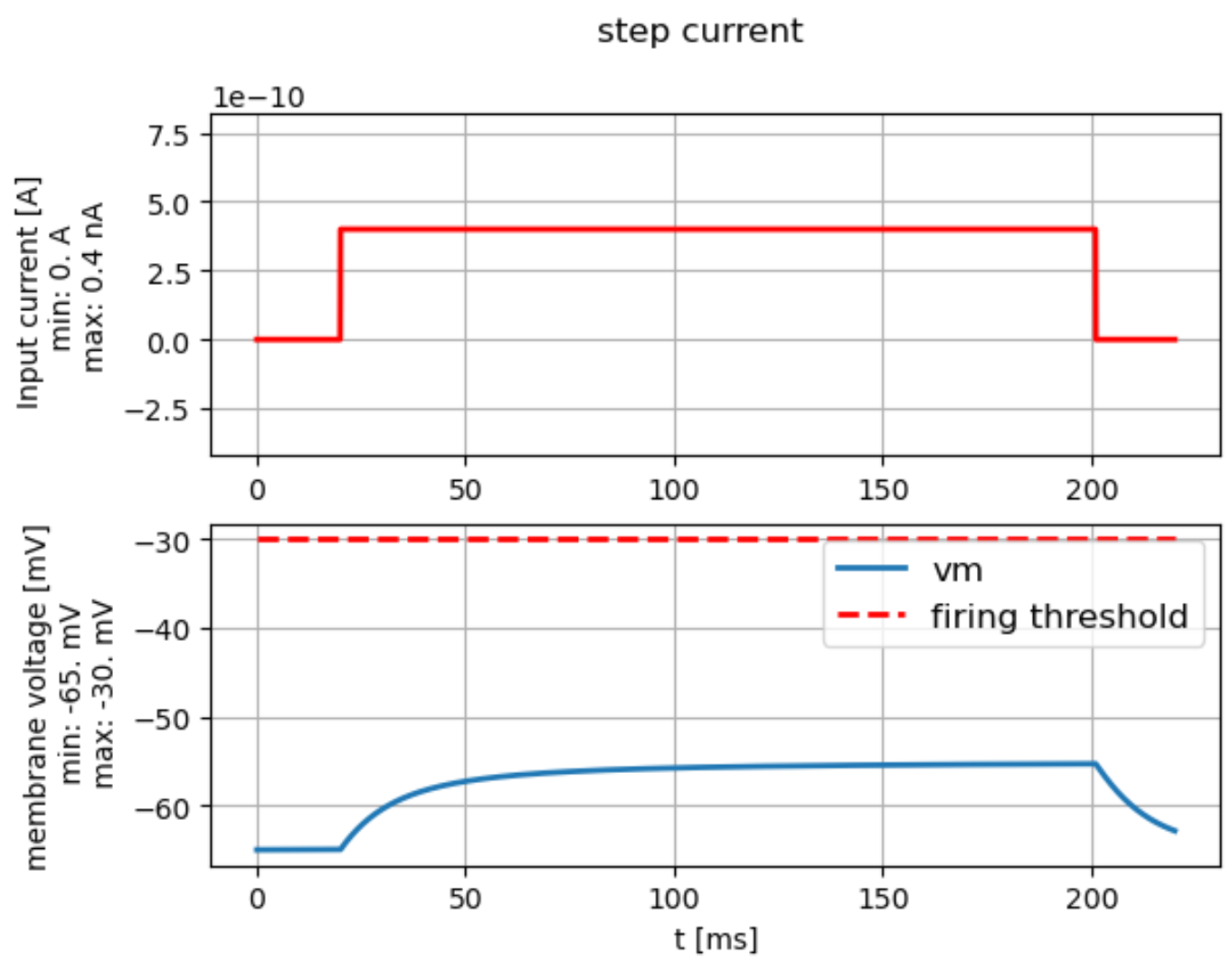
计算举例: 假设 \(\vthrh=-55\ \t{mV},\ u_\rest=-65\ \t{mV},\ \Delta_T=2\ \t{mV},\ R=20\ \t{M}\Omega\) , 则可以算得 \(I_\t{rh}= 0.4\ \t{nA}\). 可以作图验证一下该结果.

给予 \(I=0.40\ \t{nA}\) 的 step current input 时:

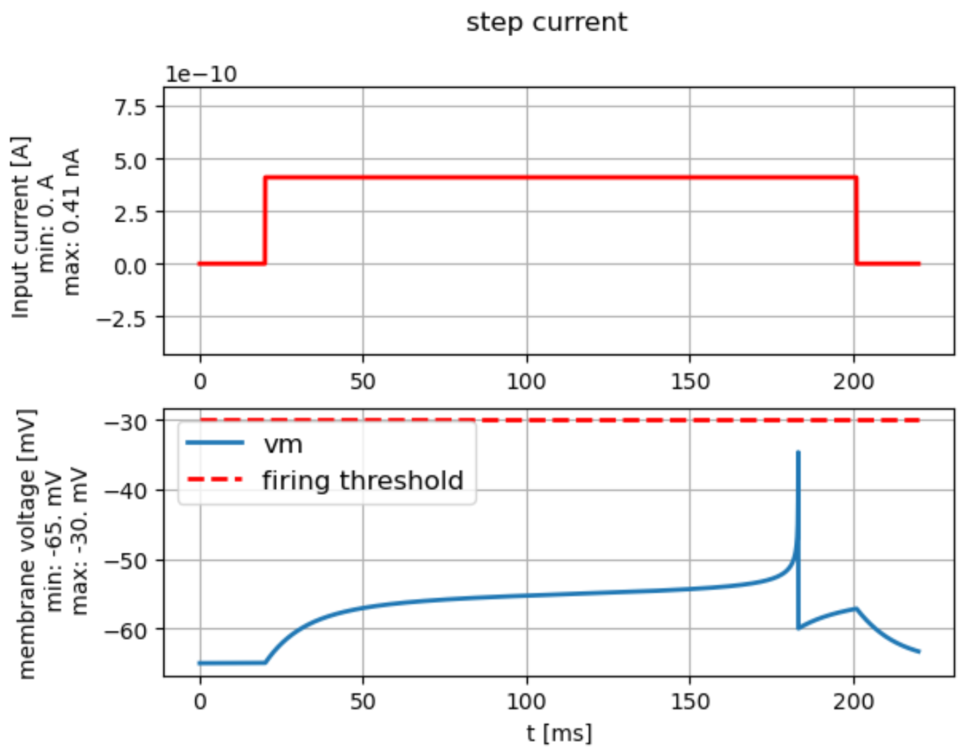
给予 \(I=0.41\ \t{nA}\) 的 step current input 时 (由于分辨率问题, 蓝色实线没有触碰到红色虚线, 实际上应该是触碰到的, 且在此时给予一个 "event". ):

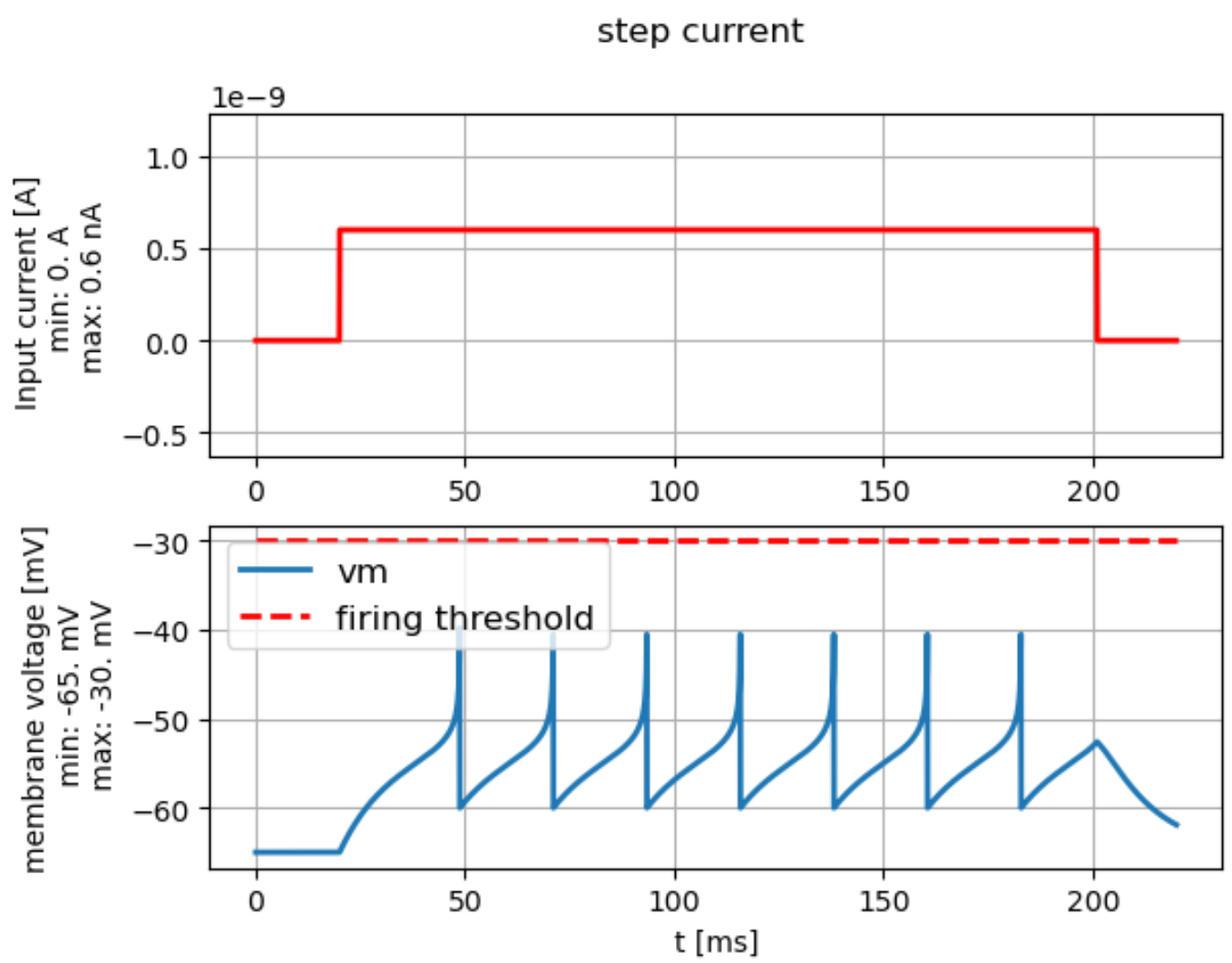
继续增大电流就有 (\(I=0.6\ \t{nA}\)):

From Hodgkin-Huxley to Exponential Integrate-and-Fire

一个自然的问题是, 凭什么 \(f(u)\) 要取 exponential 的形式? 能否与 HH model 的结果契合?

在 Chapter 4, 我们给出了 reduced to two dimensions 的 HH-model:

\[ \begin{aligned} \frac{\rmd u}{\rmd t}&=\frac{1}{\tau}[F(u,w)+RI]\\ \frac{\rmd w}{\rmd t}&=\frac{1}{\tau_w}G(u,w) \end{aligned} \]

通过适当的 scaling, 可以得到这样的简化形式:

\[ \begin{aligned} \frac{\rmd u}{\rmd t}&=F(u,w)+I\\ \frac{\rmd w}{\rmd t}&=\epsilon G(u,w) \end{aligned} \]

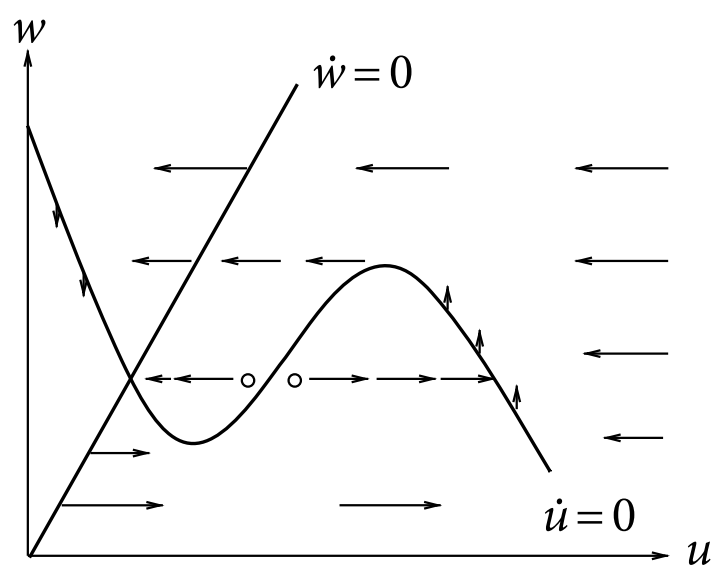
其中, \(\epsilon=\tau/\tau_w\), 可以刻画 \(u\) 和 \(w\) 动力学变化的速度. 如果 \(\tau_w \gg \tau,\ \Leftrightarrow \epsilon\ll 1\), 即 \(u\) 变化得要比 \(w\) 快得多, 那么, 在相平面上, 除了 \(\dot{u}=0\) 曲线上的流向垂直于 \(u\) 轴, 其他区域的流向几乎都与 \(u\) 轴平行. 只要不考察动作电位的起始, 即 \(u=u_\rest\) 附近, 就可以认为 \(w=w_\rest\), 如下图所示:

此时就有:

\[ \frac{\rmd u}{\rmd t}=F(u,w_\rest)+I \]

将 \(F(u,w_\rest)\) 对 \(u\) 作图结果如下:

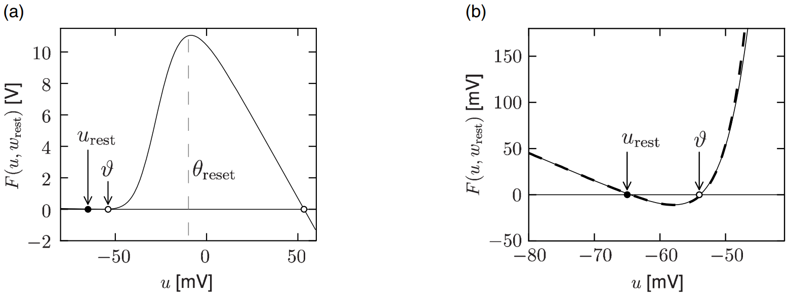
在 \(u_\rest\) 和 \(\vartheta\) 附近这段的契合度是很高的.

从 HH model 到 exponential IF, 实现了又一次降维. 这个过程中丢失了什么信息呢? 事实上, 由于 \(w\) 是用来刻画 \(h,\ n\) 的动力学特征的, 因此 \(w\) 给出了动作电位复极化的过程. 如果将 \(w\) 设置为常数, 就必须人为地设置一个 \(\theta_\text{reset}\) 作为电压能达到的 peak, 并强制使电位在达到 \(\theta_\text{reset}\) 的时刻归于 \(u_{\text{reset}}\).