\[ \newcommand{\bs}{\boldsymbol} \newcommand{\bsX}{\boldsymbol{X}} \newcommand{\bf}{\mathbf} \newcommand{\msc}{\mathscr} \newcommand{\mca}{\mathcal} \newcommand{\T}{\text{T}} \newcommand{\rme}{\mathrm{e}} \newcommand{\rmi}{\mathrm{i}} \newcommand{\rmj}{\mathrm{j}} \newcommand{\rmd}{\mathrm{d}} \newcommand{\rmm}{\mathrm{m}} \newcommand{\rmb}{\mathrm{b}} \newcommand{\and}{\land} \newcommand{\or}{\lor} \newcommand{\exist}{\exists} \newcommand{\sube}{\subseteq} \newcommand{\lr}[3]{\left#1 #2 \right#3} \newcommand{\intfy}{\int_{-\infty}^{+\infty}} \newcommand{\sumfy}[1]{\sum_{#1=-\infty}^{+\infty}} \newcommand{\vt}{\vartheta} \newcommand{\ve}{\varepsilon} \newcommand{\vp}{\varphi} \newcommand{\Var}{\text{Var}} \newcommand{\Cov}{\text{Cov}} \newcommand{\edef}{\xlongequal{def}} \newcommand{\prob}{\text{P}} \newcommand{\Exp}{\text{E}} \newcommand{\t}[1]{\text#1} \newcommand{\N}{\mathbb{N}} \newcommand{\Z}{\mathbb{Z}} \newcommand{\Q}{\mathbb{Q}} \newcommand{\R}{\mathbb{R}} \newcommand{\C}{\mathbb{C}} \newcommand{\versionofnewcommand}{\text{260125}} \]

Dimensionality Reduction and Phase Plane Analysis

Reduction to Two Dimensions

In this section, we perform a systematic reduction of the four dimensional Hodgkin-Huxley model to two dimensions. That is, two of the four variables have to be eliminated.

General Approach

首先回顾一下, Hodgkin-Huxley 模型长什么样:

\[ \begin{aligned} C\frac{\rmd u}{\rmd t} &=-\sum_k I_k+I(t)\\ \sum_kI_k &=g_{\text{Na}}m^3h(u-E_{\text{Na}})+g_{K}n^4(u-E_{\text{K}})+g_{\text{L}}(u-E_{\text{L}})\\ \frac{\rmd x}{\rmd t} &=-\frac{1}{\tau_x(u)}[x-x_0(u)] \end{aligned} \]

这里涉及了四个变量, \(m\), \(h\), \(n\), \(u\). 其中, \(m\), \(h\), \(n\) 的参数如下:

Separation of Time Scales

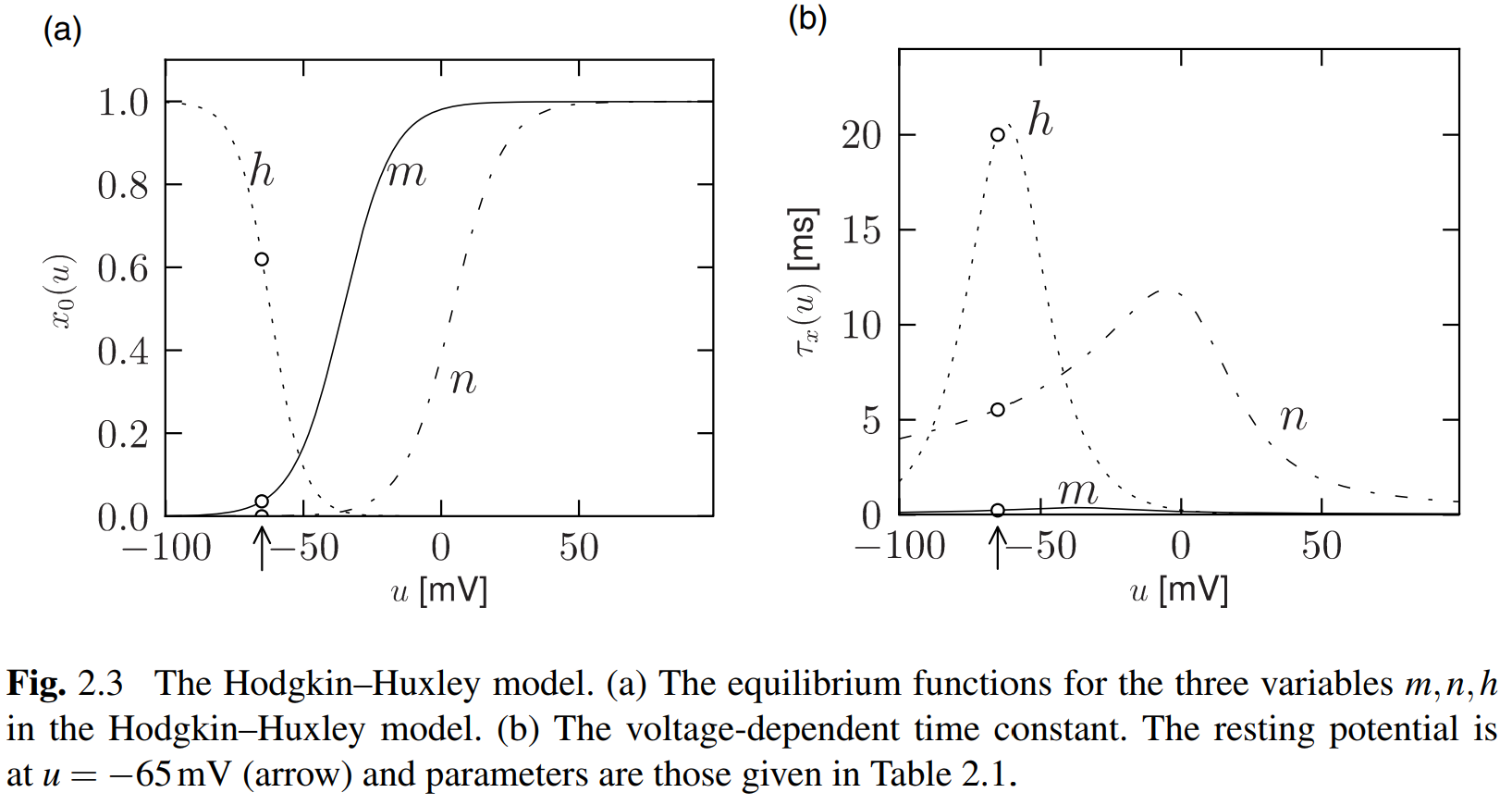
在 Fig2.3(b) 中, 可以看到, \(\tau_m\) 要远小于 \(\tau_h\) 和 \(\tau_n\). 这意味着 \(m\) 在很短的时间内就达到了 \(m_0(u)\), 从而可以认为, \(m\equiv m_0(u)\) 在所有时间上恒成立. 这样, 就消除了一个变量 \(m\).

Exploiting Similarities

The graphs of \(n_0(u)\) and \(1-h_0(u)\) have similar dynamics over the voltage \(u\), which gives a hint that these two variable can be approximated as a single effective variable \(w\). So that we set it as a linear form:

\[ \begin{aligned} w &=b-h=an\\ \Leftrightarrow h &=b-w,\ \ n=w/a \end{aligned} \]

In that case, Equation of HH model becomes:

\[ C\frac{\rmd u}{\rmd t}=-g_{\text{Na}}[{m_0(u)}]^3(b-w)(u-E_{\text{Na}})-g_{K}\left(\frac{w}{a}\right)^4(u-E_{\text{K}})-g_{\text{L}}(u-E_{\text{L}})+I(t) \]

Or, noted as:

\[ \frac{\rmd u}{\rmd t}=\frac{1}{\tau}[F(u,w)+RI] \]

​ with parameters \(R={g_\text{L}}^{-1}\), \(\tau=RC\) and some function \(F\).

​ And,

\[ \frac{\rmd w}{\rmd t}=\frac{1}{\tau_w}G(u,w) \]

​ with parameter \(\tau_w\) and function \(G\) which interpolates between \(\rmd n/\rmd t\) and \(\rmd h/\rmd t\).

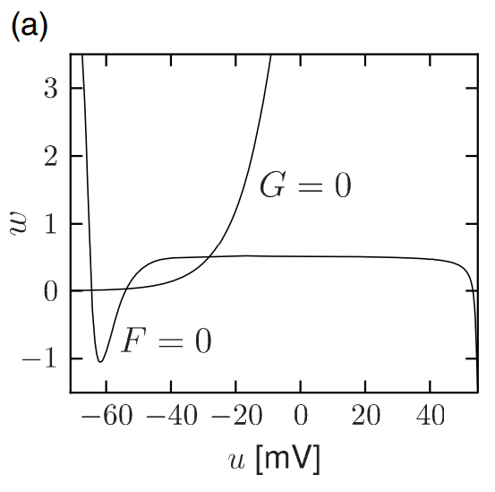
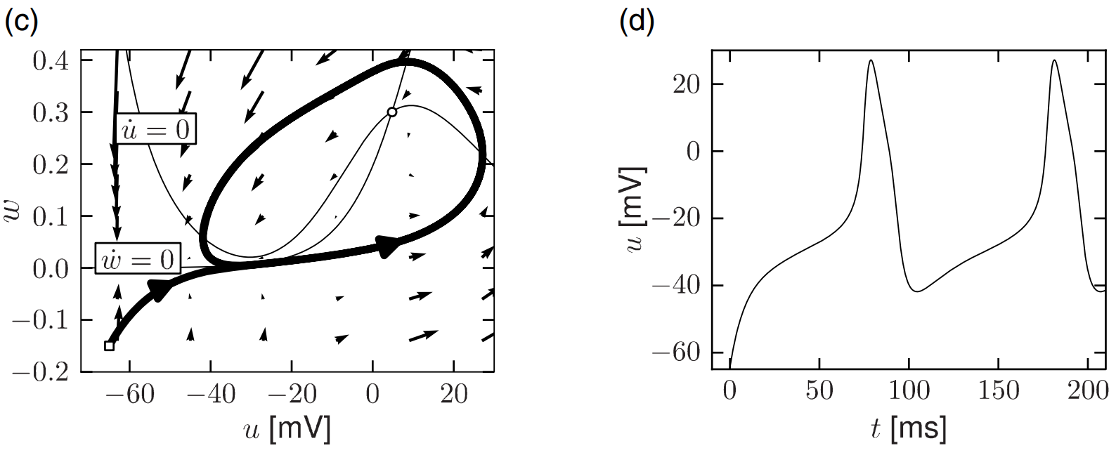
Here is the phase plane with \(u,\ w\) of a Hodgkin-Huxley model reduced to two dimensions defined above:

Mathematical Explanation

Some explanation should be discussed concerning the effectiveness of this approximation.

Consider a plane spanned by \(n\) and \(h\). If \(an(t)=b-h(t)\) establishes at each time, then all points \((n,h)\) would lie on the straight line \(h=b-an\). However, this expectation is so idealistic. The reduction of the number of variables has to be achieved by a projection of those points onto the line, and, the position along the line \(h=b-an\) gives the new variable \(w\). (\(h=b-w\)).

A simple intuition is, that the the origin of coordinate system should be set to represent the rest state:

\[ \begin{aligned} x=n-n_0(u_{\text{rest}})\\ y=h-h_0(u_{\text{rest}}) \end{aligned} \]

Although dots \((n,h)\) could be arbitrary on the two-dimensional space, these dots have a trend leading to the curve defined by all possible \(u\), that is, \((n_0(u),h_0(u))\), which is also the equilibrium values.

为了方便计算投影, 接下来要做的事是, 将坐标轴旋转一个如下定义的 \(\alpha\) 角度:

\[ \tan\alpha={\frac{\rmd h_0}{\rmd u}\Big|_{u_{\text{rest}}}}\Big/{\frac{\rmd n_0}{\rmd u}\Big|_{u_{\text{rest}}}} \]

由于坐标原点是由 \(u_{\text{rest}}\) 定义的, 这意味着旋转后的横轴就是原点的切线, 纵轴则与图像正交于原点. 新的坐标为:

\[ \begin{pmatrix} z_1\\z_2\end{pmatrix}= \begin{pmatrix} \cos\alpha & \sin\alpha\\-\sin\alpha & \cos\alpha\end{pmatrix}= \begin{pmatrix} x\\y\end{pmatrix} \]

坐标逆变换则为:

\[ \begin{pmatrix} x\\y\end{pmatrix}= \begin{pmatrix} \cos\alpha & -\sin\alpha\\ \sin\alpha & \cos\alpha\end{pmatrix}= \begin{pmatrix} z_1\\z_2\end{pmatrix} \]

把横轴, 即过 \(u_\text{rest}\) 点的切线作为投影的目标, 只需设定 \(z_2=0\). 即:

\[ \begin{aligned} &x=z_1\cos\alpha\\ \ &y=z_1\sin\alpha\\ \end{aligned} \]

因此, \((n,h)\) 在这条直线上的投影 \((n^\prime,h^\prime)\) 就是:

\[ \begin{aligned} n^\prime &=n_0(u_\text{rest})+z_1\cos\alpha\\ h^\prime &=h_0(u_\text{rest})+z_1\sin\alpha \end{aligned} \]

结合 \(n,\ h\) 关于时间的动力学方程, 有:

\[ \begin{aligned} z_1&=\cos\alpha\cdot x+\sin\alpha\cdot y\\ \Rightarrow \frac{\rmd z_1}{\rmd t}&=\cos\alpha\frac{\rmd n}{\rmd t}+\sin\alpha\frac{\rmd h}{\rmd t}\\ &=-\cos\alpha\frac{z_1\cos\alpha+n_0({u_{\text{rest}}})-n_0(u)}{\tau_n(u)}-\sin\alpha\frac{z_1\sin\alpha+h_0({u_{\text{rest}}})-h_0(u)}{\tau_h(u)} \end{aligned} \]

其实, 此时已经把 \(n,\ h\) 用一个变量 \(z_1\) 表示了. 为了得出更简洁的形式, 设:

\[ \begin{aligned} &w=-\tan\alpha\ n_0(u_{\text{rest}})-z_1\sin\alpha\\ \Rightarrow\quad& \begin{cases} &n^\prime=w/-\tan\alpha \\ &h^\prime=[-\tan\alpha\ n_0(u_{\text{rest}})+h_0(u_{\text{rest}})]-w \end{cases} \end{aligned} \]

设

\[ \begin{cases} &a=-\tan\alpha \\ &b=-\tan\alpha\ n_0(u_{\text{rest}})+h_0(u_{\text{rest}}) \end{cases} \]

则有:

\[ \begin{cases} &n^\prime=w/a \\ &h^\prime=b-w \end{cases} \]

相应地, \({\rmd w}/{\rmd t}\) 也可以从 \({\rmd z_1}/\rmd t\) 的表达式中导出. 如果定义:

\[ G(u,w)=\tau_w\cdot\frac{\rmd w}{\rmd t} \]

就得到了我们先前讨论的形式.

事实上可以进一步做简化. 如果近似认为: \(\tau_n(u)=\tau_h(u)=\tau(u)\), 那么有化简后的形式:

\[ \begin{aligned} \frac{\rmd w}{\rmd t}=&-\frac{1}{\tau(u)}[w-w_0(u)] \end{aligned}\\ \]

Morris-Lecar Model

The Morris-Lecar model read:

\[ \begin{aligned} C\frac{\rmd u}{\rmd t}&=-g_1\hat{m}_0(u)(u-V_1)-g_2\hat{w}(u-V_2)-g_\text{L}(u-V_{\text{L}}+I)\\ \frac{\rmd \hat{w}}{\rmd t}&=-\frac{1}{\tau(u)}[\hat{w}-w_0(u)]\\ m_0(u)&=\frac{1}{2}\left[1+\tanh\left(\frac{u-u_1}{u_2}\right)\right]\\ w_0(u)&=\frac{1}{2}\left[1+\tanh\left(\frac{u-u_3}{u_4}\right)\right]\\ \tau(u)&={\tau_w}/{\cosh\left(\frac{u-u_3}{2u_4}\right)} \end{aligned} \]

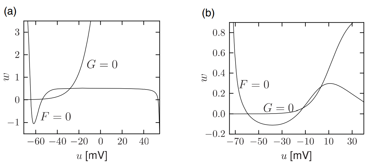
The phase plane of Morris-Lecar model is shown on the right, with that of reduction of HH model shown on the left, on contrary:

FitzHugh-Nagumo Model

The FitzHugh-Nagumo model reads:

\[ F(u,w)=u-\frac{1}{3}u^3-w\\ G(u,w)=\varepsilon (b_0+b_1u-w) \]

Phase Plan Analysis

为了分析 \(u\) 和 \(w\) 的动力学特征, 我们可以考察 \(u,\ w\) 张成的相平面. 在这里先看一下常微分方程教材里关于平面上动力系统中奇点的介绍.

Math Detour

首先考察以 \((0,0)\) 为奇点的线性系统:

\[ \frac{\rmd}{\rmd t}\begin{pmatrix}x\\y\end{pmatrix}=\boldsymbol{A}\begin{pmatrix}x\\y\end{pmatrix}\\ \boldsymbol{A}=\begin{pmatrix}a &b\\c&d\end{pmatrix} \]

Theorem: 初等奇点类型的判定

\[ \begin{aligned} &p=-\text{tr}[\boldsymbol{A}]=-(a+d)\\ &q=\det[\boldsymbol{A}]\ =ad-bc \end{aligned} \]

1) \(q<0\), \((0,0)\) 为鞍点 (saddle point) 2) \(q>0,\ p^2>4q\), \((0,0)\) 为两向结点 3) \(q>0,\ p^2=4q\), \((0,0)\) 为单向结点或星形结点 4) \(q>0,\ 0<p^2<4q\), \((0,0)\) 为焦点 5) \(q>0,\ p=0\), \((0,0)\) 为中心点.

在情形 2~4 中, 当 \(p>0\) 时奇点 \((0,0)\) 稳定, \(p<0\) 时不稳定.

Nullclines

The set of points with \({\rmd u}/{\rmd t}=0\) is called the \(u\)-nullcline. 这条线上 flow 的方向始终垂直于 \(u\)-axis. \(w\)-nullcline 也是同样的定义. 两条 nullcline 的交点就是 fixed points. 把 fixed point 平移到原点, 则平面上任一点:

\[ \boldsymbol{x}=(u-u_{FP},w-w_{FP})^{\text{T}} \]

进而可以用下式表达该线性系统:

\[ \frac{\rmd}{\rmd t}\boldsymbol{x}= \begin{pmatrix} F_u & F_w\\G_u& G_w \end{pmatrix}\boldsymbol{x} \]

从而可以由此判别奇点类型及其稳定性.

Type \(\mathrm{I}\) and Type \(\mathrm{II}\) Neuron Models

Type \(\mathrm{I}\) Models and Saddle-Node-Onto-Limit-Cycle Bifurcation

Neuron models with a continuous gain function are called type \(\mathrm{I}\). Mathematically, a saddle-node-onto-limit-cycle bifurcation generically gives rise to a type I behavior.

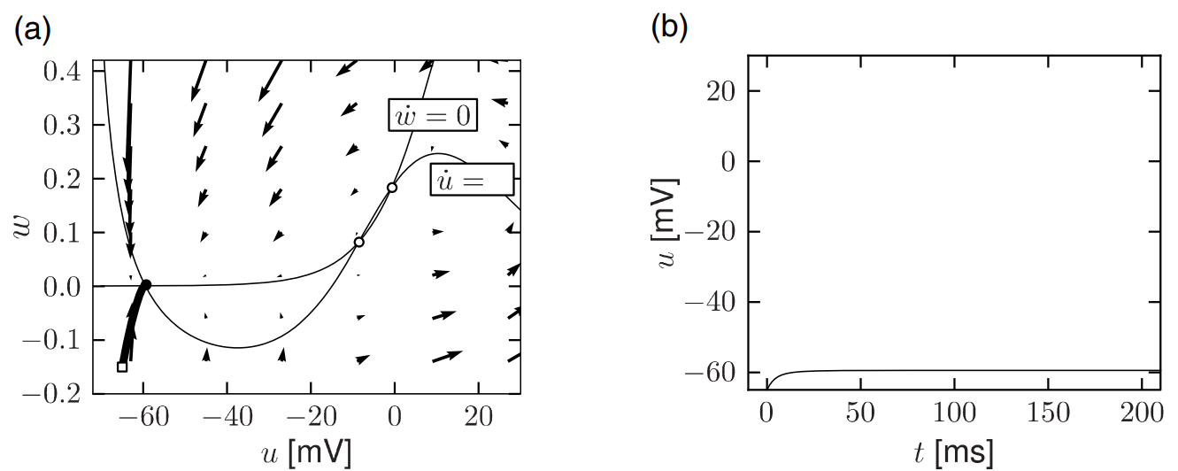
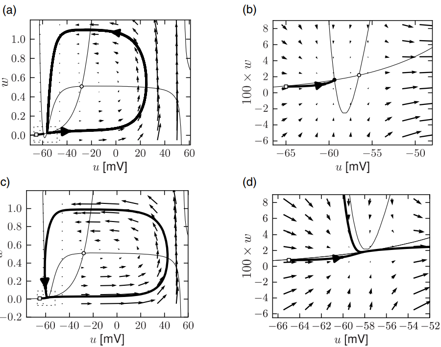
当没有额外的电流 input 时, Type \(\mathrm{I}\) neuron 在相平面中有三个奇点. 如下面的 (a) 图所示: 最左边的是稳定奇点, 中间的是鞍点 (saddle point), 最右边是不稳定奇点. 图 (b) 则是 图 (a) 中左下角黑线所示轨迹对应的电压随时间的变化. 容易看出, 电压在不够大时, 会随时间回到静息电位 \(u_{\text{rest}}\) (图中约为 \(-60\text{mV}\)) .

如果给予恒定电流输入 \(I\), \(u\) 的动力学方程中会多出一个 \(RI\) 常数项, 使得 \(\dot{u}\) 的图像向上平移. 这会导致稳定奇点与鞍点互相靠近, 直到重合, 随后消失. 如下图 (c) 中所示. 这样, 在剩下的这个不稳定奇点周围, 就会有极限环生成. 值得强调的是, 在 Type \(\mathrm{I}\) neuron 中, 稳定奇点与鞍点重合的位置 locates in 极限环内部. 因此, 这个 scenario 被称为 saddle-node-onto-limit-cycle bifurcation. 相应地, 在 图 (d) 所示的 \(u-t\) 图像中, 就会形成一个周期放电的形式.

聪明的, 你告诉我, 神经放电的频率可以用什么来刻画呢? 诶对喽, 就是极限环上转圈的频率嘛. 当 input \(I\) 等于临界电流 \(I_\theta\), 即, 两个奇点刚好消失; 那么, 围绕着这个湮灭点, 就会出现一个速度为 \(0\) 的极限环. 随着电流增大, 转圈的频率从 \(0\) 开始逐渐增大, 这符合在先前的章节中对 Type \(\mathrm{I}\) 的定义: Neuron models with a continuous gain function (\(f-I\) curve).

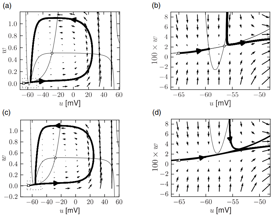
上面给出的两张图是适当选取参数后的 Morris-Lecar Model; 事实上, 通过调整参数, 该模型可以变成 Type \(\mathrm{II}\) neuron. 同样地, 调整 reduced HH model 的参数也可以使它成为 Type \(\mathrm{I}\) 或 Type \(\mathrm{II}\). 其相平面图如下所示:

Type \(\mathrm{II}\) Models and Saddle-Node-Off-Limit-Cycle Bifurcation

呃, 尽管我不甚清楚其数学原理, 但书中说, 极限环的生成不一定要伴随着奇点消失, 它完全可以在两奇点湮灭前就已经存在, 如下图中的情况. 此时, 放电频率不再是从 \(0\) 开始逐渐增大. 可是, 呃, 为什么呢? 我不太理解.

Threshold and Excitability

从上一节的讨论中, 我们发现, 对于 models with saddle-node-bifurcation, 无论是 on 还是 off limit cycle, 都是有 threshold 的; 但 Hopf bifurcation 却没有.

tbc...